


WHEN THERE ISN'T WAP THAN WRITE ONLY ALGORITHM WILL DO.
ANS
1.
i. Recursion is a process in which the problem is specified in terms of itself.
ii. The function should be called itself to implement recursion.
iii. The function which calls itself is called as recursive function.
iv. A condition must be specified to stop recursion; otherwise it will lead to an infinite process.
v. In case of recursion, all partial solutions are combined to obtain the final solution.
vi. Example: Factorial of a number
2. Advantages:
i. The main benefit of a recursive approach to algorithm design is that it allows programmers to take advantage of the repetitive structure present in many problems.
ii. Complex case analysis and nested loops can be avoided.
iii. Recursion can lead to more readable and efficient algorithm descriptions.
iv. Recursion is also a useful way for defining objects that have a repeated similar structural form.
3. Disadvantages:
i. Slowing down execution time and storing on the run-time stack more things than required in a non recursive approach are major limitations of recursion.
ii. If recursion is too deep, then there is a danger of running out of space on the stack and ultimately program crashes.
iii. Even if some recursive function repeats the computations for some parameters, the run time can be prohibitively long even for very simple cases.
ANS 2.
Majorly, we use THREE types of Asymptotic Notations and those are as follows...
-
Big - Oh (O)
-
Big - Omega (Ω)
-
Big - Theta (Θ)
Big - Oh Notation (O)
Big - Oh notation is used to define the upper bound of an algorithm in terms of Time Complexity.That means Big - Oh notation always indicates the maximum time required by an algorithm for all input values. That means Big - Oh notation describes the worst case of an algorithm time complexity.
Big - Oh Notation can be defined as follows...
Consider function f(n) the time complexity of an algorithm and g(n) is the most significant term. If f(n) <= C g(n) for all n >= n0, C > 0 and n0 >= 1. Then we can represent f(n) as O(g(n)).
f(n) = O(g(n))
Consider the following graph drawn for the values of f(n) and C g(n) for input (n) value on X-Axis and time required is on Y-Axis

Example
Consider the following f(n) and g(n)...f(n) = 3n + 2
g(n) = n
If we want to represent f(n) as O(g(n)) then it must satisfy f(n) <= C x g(n) for all values of C > 0 and n0>= 1
f(n) <= C g(n)
⇒3n + 2 <= C n
Above condition is always TRUE for all values of C = 4 and n >= 2.
By using Big - Oh notation we can represent the time complexity as follows...
3n + 2 = O(n)
Big - Omege Notation (Ω)
Big - Omega notation is used to define the lower bound of an algorithm in terms of Time Complexity.That means Big - Omega notation always indicates the minimum time required by an algorithm for all input values. That means Big - Omega notation describes the best case of an algorithm time complexity.
Big - Omega Notation can be defined as follows...
Consider function f(n) the time complexity of an algorithm and g(n) is the most significant term. If f(n) >= C x g(n) for all n >= n0, C > 0 and n0 >= 1. Then we can represent f(n) as Ω(g(n)).
f(n) = Ω(g(n))
Consider the following graph drawn for the values of f(n) and C g(n) for input (n) value on X-Axis and time required is on Y-Axis

Example
Consider the following f(n) and g(n)...f(n) = 3n + 2
g(n) = n
If we want to represent f(n) as Ω(g(n)) then it must satisfy f(n) >= C g(n) for all values of C > 0 and n0>= 1
f(n) >= C g(n)
⇒3n + 2 <= C n
Above condition is always TRUE for all values of C = 1 and n >= 1.
By using Big - Omega notation we can represent the time complexity as follows...
3n + 2 = Ω(n)
Big - Theta Notation (Θ)
Big - Theta notation is used to define the average bound of an algorithm in terms of Time Complexity.That means Big - Theta notation always indicates the average time required by an algorithm for all input values. That means Big - Theta notation describes the average case of an algorithm time complexity.
Big - Theta Notation can be defined as follows...
Consider function f(n) the time complexity of an algorithm and g(n) is the most significant term. If C1 g(n) <= f(n) >= C2 g(n) for all n >= n0, C1, C2 > 0 and n0 >= 1. Then we can represent f(n) as Θ(g(n)).
f(n) = Θ(g(n))
Consider the following graph drawn for the values of f(n) and C g(n) for input (n) value on X-Axis and time required is on Y-Axis

ANS 3.
Array Vs Linked List
Comparison Chart
|
Basis for Comparison |
Array |
Linked list |
|---|---|---|
|
Basic |
It is a consistent set of a fixed number of data items. |
It is an ordered set consisting of a variable number of data
items. |
|
Size |
Specified during declaration. |
No need to specify; grow and shrink during execution.
|
|
Storage Allocation
|
Element location is allocated during compile time. |
Element position is assigned during run time. |
|
Order of the elements
|
Stored consecutively
|
Stored randomly |
|
Accessing the element |
Direct or randomly accessed, i.e., Specify the array index or
subscript. |
Sequentially accessed, i.e., Traverse starting from the first
node in the list by the pointer. |
|
Insertion and deletion of element |
Slow relatively as shifting is required. |
Easier, fast and efficient.
|
|
Searching
|
Binary search and linear search |
linear search |
|
Memory required |
less
|
More
|
|
Memory Utilization |
Ineffective |
Efficient
|
ANS 4.
ADT
-
An abstract data type (ADT) is basically a logical description or a specification of components of the data and the operations that are allowed, that is independent of the implementation.
ADTs are a theoretical concept in computer science, used in the design and analysis of algorithms, data structures, and software systems, and do not correspond to specific features of computer languages.
There may be thousands of ways in which a given ADT can be implemented, even when the coding language remains constant. Any such implementation must comply with the content-wise and behavioral description of the ADT.
Examples
For example, integers are an ADT, defined as the values 0, 1, −1, 2, 2, ..., and by the operations of addition, subtraction, multiplication, and division, together with greater than, less than, etc. which are independent of how the integers are represented by the computer. Typically integers are represented in as binary numbers, most often as two's complement, but might be binary-coded decimal or in ones' complement, but the user is abstracted from the concrete choice of representation, and can simply use the data as integers.
Another example can be a list, with components being the number of elements and the type of the elements. The operations allowed are inserting an element, deleting an element, checking if an element is present, printing the list etc. Internally, we may implement list using an array or a linked list, and hence the user is abstracted from the concrete implementation.
ANS 5.
Linear Data Structure:
-
Those data structures where the data elements are organised in some sequence is called linear data structure.
-
Here the various operations on a data structure are possible only in a sequence i.e. we cannot insert the element into any location of our choice. E.g. A new element in a queue can come only at the end, not anywhere else.
-
Examples of linear data structures are array, stacks, queue, and linked list.
-
They can be implemented in memory using two ways.
-
The first method is by having a linear relationship between elements by means of sequential memory locations.
-
The second method is by having a linear relationship by
using links.
Non-Linear Data Structure:
-
When the data elements are organised in some arbitrary
function without any sequence, such data structures are called
non-linear data structures.
-
Examples of such type are trees, graphs.
-
The relationship of adjacency is not maintained between
elements of a non-linear data structure.
Graph data structure is represented using following representations...
-
Adjacency Matrix
-
Incidence Matrix
-
Adjacency List
Adjacency Matrix
In this representation, graph can be represented using a matrix of size total number of vertices by total number of vertices. That means if a graph with 4 vertices can be represented using a matrix of 4X4 class. In this matrix, rows and columns both represents vertices. This matrix is filled with either 1 or 0. Here, 1 represents there is an edge from row vertex to column vertex and 0 represents there is no edge from row vertex to column vertex.For example, consider the following undirected graph representation...


Incidence Matrix
In this representation, graph can be represented using a matrix of size total number of vertices by total number of edges. That means if a graph with 4 vertices and 6 edges can be represented using a matrix of 4X6 class. In this matrix, rows represents vertices and columns represents edges. This matrix is filled with either 0 or 1 or -1. Here, 0 represents row edge is not connected to column vertex, 1 represents row edge is connected as outgoing edge to column vertex and -1 represents row edge is connected as incoming edge to column vertex.For example, consider the following directed graph representation...

Adjacency List
In this representation, every vertex of graph contains list of its adjacent vertices.For example, consider the following directed graph representation implemented using linked list...


An arithmetic expression such as (5-x)*y+6/(x + z) is a combination of arithmetic operators (+, -, *, /, etc.), operands (5, x, y, 6, z, etc.), and parentheses to override the precedence of operations.
-
Each expression can be represented by a unique binary tree whose structure is determined by the precedence of operation in the expression. Such a tree is called an expression tree.
-
Algorithm for building expression tree: a. The expression tree for a given expression can be built recursively from the following rules: i. The expression tree for a single operand is a single root node that contains it. ii. If E1 and E2 are expressions represented by expression trees T1 and T2, and if op is an operator, then the expression tree for the expression El op E2 is the tree with the root node containing op and sub-trees T1 and T2. b. An expression has three representations, depending upon which traversal algorithms are used to traverse its tree. The preorder traversal produces the prefix representation, the in-order traversal produces the infix representation, and the post-order traversal produces the postfix representation of the expression. The postfix representation is also called reverse Polish notation or RPN.
-
Example of an expression tree: Here is the expression tree
for the expression: (5-x)*y+6/(x + z)

(NOTE - YOU MUST FOLLOW YOUR CLASS NOTEBOOK FOR PROGRAM)
#include#includestruct node *insert begin(struct node *start){Struct node *new_node;int num;printf("\n enter the value");scanf("%d",&num);new_node=(struct node *)malloc(sizeof(struct node));new_node->data=num;start->prev=new_node;new_node->next=start;new->prev=NULL;start=new_node;return start;}struct node *insert_end(struct node *start){struct node *new_node,*ptr;ptr=start;int num;printf("\n enter the value");scanf("%d",&num);new_node=(struct node *)malloc(sizeof(struct node));new_node->data=num;while(ptr->next!=NULL){ptr=ptr->next;}ptr->next=new_node;start->prev=new_node;new_node->next=NULL;new->prev=ptr;return start;}struct node *delete_begin(struct node *start){struct node *ptr;ptr=start;start=start->next;start=start->prev;free(ptr);return start;}struct node *delete_end(struct node *start){struct node *ptr;ptr=start;while(ptr->next!=NULL){ptr=ptr->next;}ptr->prev->next=NULL;free(ptr);return start;}struct node *create_linked_list(struct node *start){struct node *new_node,*ptr;int num;printf("\n Enter the data:");scanf("%d",&num);while(num!=-1){if(start==NULL){new_node=(struct node*)malloc(sizeof(struct node));new_node->prev=NULL;new_node->data=num;new_node->next=NULL;start=new_node;}else{ptr=start;new_node=(struct node*)malloc(sizeof*struct node));new_node->data=num;while(ptr->next!=NULL){ptr=ptr->next;}ptr->next=new_node;new_node->prev=ptr;new_node->next=NULL;}printf("\n Enter next data:");scanf("%d",&num);}return start;}struct node{struct node *next;struct node *prev;int data;};struct node *start=NULL;int main(){int choice;printf("\n 1. create linked list");printf("\n 2. add in beginning");printf("\n 3. add at end");printf("\n 4. delete from beginning");printf("\n 5. delete from end");scanf("%d",&choice);switch(choice){case 1:start=create_linked_list(start);break;case 2: start=insert_begin(start);break;case 3:start=insert_end(start);break;case 4:start=delete_begin(start);break;case 5:start=delete_end(start);break;}return0;}
#includeSample Output:#includeusing namespace std;class Stack{int stk[10];int top;public:Stack(){top=-1;}//This funtion is used to push an elemnt into stackvoid push(int x){if(isFull()){cout <<"Stack is full";return;}top++;stk[top]=x;cout <<"Inserted Element:"<<" "<}//This functionn is used to check if the stack is fullbool isFull(){int size=sizeof(stk)/sizeof(*stk);if(top == size-1){return true;}else{return false;}}//This function is used to check if the stack is emptybool isEmpty(){if(top==-1){return true;}else{return false;}}//This function is used to pop an element of stackvoid pop(){if(isEmpty()){cout <<"Stack is Empty";return;}cout <<"Deleted element is:" <<" "<}//This function is used to display the elements of the stackvoid display(){if(top==-1){cout <<" Stack is Empty!!";return;}for(int i=top;i>=0;i--){cout <}}};void main(){int ch;Stack st;while(1){cout <<"\n1.Push 2.Pop 3.Display 4.Exit\nEnter ur choice";cin >> ch;switch(ch){case 1: cout <<"Enter the element you want to push";cin >> ch;st.push(ch);break;case 2: st.pop();break;case 3: st.display();break;case 4: exit(0);}}}
ANS 10.1.Push 2.Pop 3.Display 4.ExitEnter ur choice 1Enter the element you want to push 11Inserted Element: 111.Push 2.Pop 3.Display 4.ExitEnter ur choice 1Enter the element you want to push 22Inserted Element: 221.Push 2.Pop 3.Display 4.ExitEnter ur choice 1Enter the element you want to push 33Inserted Element: 331.Push 2.Pop 3.Display 4.ExitEnter ur choice 1Enter the element you want to push 44Inserted Element: 441.Push 2.Pop 3.Display 4.ExitEnter ur choice 1Enter the element you want to push 55Inserted Element: 551.Push 2.Pop 3.Display 4.ExitEnter ur choice 355 44 33 22 111.Push 2.Pop 3.Display 4.ExitEnter ur choice 2Deleted element is: 551.Push 2.Pop 3.Display 4.ExitEnter ur choice 344 33 22 111.Push 2.Pop 3.Display 4.ExitEnter ur choice
//
program to implement queue using array#include#define MAX 10 /* The maximum size of the queue */#includevoid insert(int queue[], int *rear, int value){if(*rear < MAX-1){*rear= *rear +1;queue[*rear] = value;}else{printf("The queue is full can not insert a value\n");exit(0);}}void delete(int queue[], int *front, int rear, int * value){if(*front == rear){printf("The queue is empty can not delete a value\n");exit(0);}*front = *front + 1;*value = queue[*front];}void main(){int queue[MAX];int front,rear;int n,value;front=rear=(-1);do{do{printf("Enter the element to be inserted\n");scanf("%d",&value);insert(queue,&rear,value);printf("Enter 1 to continue\n");scanf("%d",&n);}while(n == 1);printf("Enter 1 to delete an element\n");scanf("%d",&n);while( n == 1){delete(queue,&front,rear,&value);printf("The value deleted is %d\n",value);printf("Enter 1 to delete an element\n");scanf("%d",&n);}printf("Enter 1 to continue\n");scanf("%d",&n);}while(n == 1);}
ANS 11.
In infix expressions, the operator precedence is implicit unless we use parentheses. Therefore, for the infix to postfix conversion algorithm, we have to define the operator precedence inside the algorithm. We did this in the post covering infix, postfix and prefix expressions.
THE ALGORITHM:-
-
Create a stack
-
for each character ‘t’ in the input stream {
-
if (t is an operand)
output t -
else if (t is a right parentheses){
POP and output tokens until a left parentheses is popped(but do not output)
} -
else {
POP and output tokens until one of lower priority than t is encountered or a left parentheses is encountered
or the stack is empty
PUSH t
}
-
-
POP and output tokens until the stack is empty.
|
INPUT CHARACTER |
OPERATION ON STACK |
STACK |
POSTFIX EXPRESSION |
|
A |
Empty |
A |
|
|
* |
Push |
* |
A |
|
B |
* |
A B |
|
|
– |
Check and Push |
– |
A B * |
|
( |
Push |
– ( |
A B * |
|
C |
– ( |
A B * C |
|
|
+ |
Check and Push |
– ( + |
A B * C |
|
D |
– ( + |
A B * C D |
|
|
) |
Pop and append to postfix till ‘(‘ |
– |
A B * C D + |
|
+ |
Check and push |
+ |
A B * C D + – |
|
E |
+ |
A B * C D + – E |
|
|
End of Input |
Pop till Empty |
Empty |
A B * C D + – E + |
OR
Algorithm to convert from infix to prefix:
-
START
-
INPUT the expression EXPR from the user.
-
Reverse the EXPR obtained in step 1 to obtain REVEXPR. While reversing the string interchange the right and left parentheses. REVEXPR → REVERSE(EXPR)
-
Calculate the POSTFIX expression of the reversed string. POSTFIXEXPR → POSTFIX(REVEXPR)
-
Reverse the POSTFIXEXPR to obtain the Prefix expression PREFIXEXPR. PREFIXEXPR→ REVERSE(POSTFIXEXPR)
-
STOP
ANS 12.
-
In Queue, the insertion and deletion takes place by the FIFO policy. However, in priority queue, the insertion and deletion takes place based on the priority assigned to each element.
-
It is a special type of queue where if an element needs to be taken out from the queue, we remove the highest-priority element.
-
The general rule regarding evaluation of priority queue are:
-
The elements of high priority are processed before the elements of lower priority.
-
If the priority values are same, we apply FCFS principle.
-
-
Priority queues are widely used in operating systems. The
value of priority can be based on various factors like CPU time
required, memory requirement etc.
-
Priority queues can represented in two ways.
-
Array or Sequential representation.
-
Dynamic or linked representation.
-
-
ALGO OF PRIORITY QUEUE -
void insert(int data){
   int i = 0;

   if(!isFull()){
      // if queue is empty, insert the data

      if(itemCount == 0){
         intArray[itemCount++] = data;
      }else{
         // start from the right end of the queue
         for(i = itemCount - 1; i >= 0; i-- ){
            // if data is larger, shift existing item to right end
            if(data > intArray[i]){
               intArray[i+1] = intArray[i];
            }else{
               break;
            }
         }
         // insert the data
         intArray[i+1] = data;
         itemCount++;
      }
   }
}
QUICK SORT
QuickSort(array,begin,end)
i. If (begin
a. divide(array,begin,end,pivot)
b. quickSort(array,begin,pivot-1)
c. quicksort(array,pivot+1,end)
d. END IF ii. STOP
Divide(array,begin,end,pivot)
i. Set Left=Begin , Right=End, pivot=begin
ii. Initialize flag to false.
iii. While Flag=false.
a. While array[pivot]<=array[right] and pivot≠right.
Decrement right by 1.
b. If pivot=right
Set Flag=True.
c. Else if array[pivot]>array[right]
Swap array[pivot] and array[right].
Set right pointer as pivot.
d. If flag=false
-
While array[pivot]>=array[left] and pivot≠left
-
IF pivot=left
Set Flag=false.
-
Else if array[pivot]
Set left pointer as pivot.
iv. Return pivot position.
-
Let us assume that T(n) be the complexity and that all
elements are distinct. Recurrence for T(n) depends only on two
subproblem sizes which depend on partition element. If pivot is ith
smallest element, then exactly (i-1) items will be in the left part
and (n-i) in the right part. Since each element has equal
probability of being selected as pivot, the probability of selecting
ith element is 1/n.
-
In best case: each partition splits array in halves.
-
In worst case: Each partition gives unbalanced spilt.
SELECTION SORT
Algorithm
Step 1 − Set MIN to location 0
Step 2 − Search the minimum element in the list
Step 3 − Swap with value at location MIN
Step 4 − Increment MIN to point to next element
Step 5 − Repeat until list is sorted
Pseudocode
procedure selection sort
   list  : array of items
   n     : size of list

   for i = 1 to n - 1
   /* set current element as minimum*/
      min = i

      /* check the element to be minimum */

      for j = i+1 to n
         if list[j] < list[min] then
            min = j;
         end if
      end for

      /* swap the minimum element with the current element*/
      if indexMin != i  then
         swap list[min] and list[i]
      end if

   end for

end procedure
INSERTION
SORTAlgorithm
Now we have a bigger picture of how this sorting technique works, so we can derive simple steps by which we can achieve insertion sort.Step 1 − If it is the first element, it is already sorted. return 1;
Step 2 − Pick next element
Step 3 − Compare with all elements in the sorted sub-list
Step 4 − Shift all the elements in the sorted sub-list that is greater than the
value to be sorted
Step 5 − Insert the value
Step 6 − Repeat until list is sorted
Pseudocode
procedure insertionSort( A : array of items )
   int holePosition
   int valueToInsert

   for i = 1 to length(A) inclusive do:

      /* select value to be inserted */
      valueToInsert = A[i]
      holePosition = i

      /*locate hole position for the element to be inserted */

      while holePosition > 0 and A[holePosition-1] > valueToInsert do:
         A[holePosition] = A[holePosition-1]
         holePosition = holePosition -1
      end while

      /* insert the number at hole position */
      A[holePosition] = valueToInsert

   end for

end procedure
BUBBLED
SORTAlgorithm
We assume list is an array of n elements. We further assume that swap function swaps the values of the given array elements.begin BubbleSort(list)
for all elements of list
if list[i] > list[i+1]
swap(list[i], list[i+1])
end if
end for
return list
end BubbleSort
Pseudocode
We observe in algorithm that Bubble Sort compares each pair of array element unless the whole array is completely sorted in an ascending order. This may cause a few complexity issues like what if the array needs no more swapping as all the elements are already ascending.To ease-out the issue, we use one flag variable swapped which will help us see if any swap has happened or not. If no swap has occurred, i.e. the array requires no more processing to be sorted, it will come out of the loop.
Pseudocode of BubbleSort algorithm can be written as follows −
procedure bubbleSort( list : array of items )

   loop = list.count;

   for i = 0 to loop-1 do:
      swapped = false

      for j = 0 to loop-1 do:

         /* compare the adjacent elements */
         if list[j] > list[j+1] then
            /* swap them */
            swap( list[j], list[j+1] )
            swapped = true
         end if

      end for

      /*if no number was swapped that means
      array is sorted now, break the loop.*/

      if(not swapped) then
         break
      end if

   end for

end procedure return list
MERGE
SORTAlgorithm
Merge sort keeps on dividing the list into equal halves until it can no more be divided. By definition, if it is only one element in the list, it is sorted. Then, merge sort combines the smaller sorted lists keeping the new list sorted too.
Step 1 − if it is only one element in the list it is already sorted, return.
Step 2 − divide the list recursively into two halves until it can no more be divided.
Step 3 − merge the smaller lists into new list in sorted order.
Pseudocode
We shall now see the pseudocodes for merge sort functions. As our algorithms point out two main functions − divide & merge.Merge sort works with recursion and we shall see our implementation in the same way.
procedure mergesort( var a as array )
   if ( n == 1 ) return a

   var l1 as array = a[0] ... a[n/2]
   var l2 as array = a[n/2+1] ... a[n]

   l1 = mergesort( l1 )
   l2 = mergesort( l2 )

   return merge( l1, l2 )
end procedure

procedure merge( var a as array, var b as array )

   var c as array

   while ( a and b have elements )
      if ( a[0] > b[0] )
         add b[0] to the end of c
         remove b[0] from b
      else
         add a[0] to the end of c
         remove a[0] from a
      end if
   end while

   while ( a has elements )
      add a[0] to the end of c
      remove a[0] from a
   end while

   while ( b has elements )
      add b[0] to the end of c
      remove b[0] from b
   end while

   return c

end procedure
ANSLYSIS
OF TIME
|
Time |
|||||||
|---|---|---|---|---|---|---|---|
|
Sort |
Average |
Best |
Worst |
Space |
Stability |
Remarks |
|
|
Bubble
sort |
O(n^2) |
O(n^2) |
O(n^2) |
Constant |
Stable |
Always use a modified bubble sort |
|
|
Modified
Bubble sort |
O(n^2) |
O(n) |
O(n^2) |
Constant |
Stable |
Stops after reaching a sorted array |
|
|
Selection
Sort |
O(n^2) |
O(n^2) |
O(n^2) |
Constant |
Stable |
Even a perfectly sorted input requires scanning the entire
array |
|
|
Insertion
Sort |
O(n^2) |
O(n) |
O(n^2) |
Constant |
Stable |
In the best case (already sorted), every insert requires
constant time |
|
|
Heap
Sort |
O(n*log(n)) |
O(n*log(n)) |
O(n*log(n)) |
Constant |
Instable |
By using input array as storage for the heap, it is possible to
achieve constant space |
|
|
Merge
Sort |
O(n*log(n)) |
O(n*log(n)) |
O(n*log(n)) |
Depends |
Stable |
On arrays, merge sort requires O(n) space; on linked lists,
merge sort requires constant space |
|
|
Quicksort |
O(n*log(n)) |
O(n*log(n)) |
O(n^2) |
Constant |
Stable |
Randomly picking a pivot value (or shuffling the array prior to
sorting) can help avoid worst case scenarios such as a perfectly
sorted array |
|
ANS 14.
Insertion in Binary Search Tree:
-
*
 A utility function to insert a new node with given key in BST */
struct
node* insert(struct node*
node, int key){ /*
If the tree is empty, return a new node */ if
(node == NULL) return newNode(key); /*
Otherwise, recur down the tree */ if
(key < node->key) node->left
= insert(node->left, key); else
if (key >
node->key) node->right
= insert(node->right, key);
/*
return the (unchanged) node pointer */
return
node;}*
Given a binary search tree and a key, this function deletes the key and
returns the new root */struct
node* deleteNode(struct node*
root, int key){ //
base case if
(root == NULL) return root; //
If the key to be deleted is smaller than the root's key, //
then it lies in left subtree if
(key < root->key) root->left
= deleteNode(root->left, key); //
If the key to be deleted is greater than the root's key, //
then it lies in right subtree else
if (key >
root->key) root->right
= deleteNode(root->right, key); //
if key is same as root's key, then This is the node //
to be deleted else { //
node with only one child or no child if
(root->left == NULL) { struct
node *temp = root->right; free(root); return
temp; } else
if (root->right
== NULL) { struct
node *temp = root->left; free(root); return
temp; } //
node with two children: Get the inorder successor (smallest //
in the right subtree) struct
node* temp = minValueNode(root->right); //
Copy the inorder successor's content to this node root->key
= temp->key; //
Delete the inorder successor root->right
= deleteNode(root->right, temp->key); } return
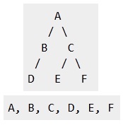
root;}ANS 15. Depth First Traversals: (a) Inorder (Left, Root, Right) : 4 2 5 1 3 (b) Preorder (Root, Left, Right) : 1 2 4 5 3 (c) Postorder (Left, Right, Root) : 4 5 2 3 1Breadth First or Level Order Traversal : 1 2 3 4 5
Please see this post for Breadth First Traversal.
Inorder Traversal:
Algorithm Inorder(tree)
   1. Traverse the left subtree, i.e., call Inorder(left-subtree)
   2. Visit the root.
   3. Traverse the right subtree, i.e., call Inorder(right-subtree)
Uses of Inorder
In case of binary search trees (BST), Inorder traversal gives nodes in non-decreasing order. To get nodes of BST in non-increasing order, a variation of Inorder traversal where Inorder itraversal s reversed, can be used.
Example: Inorder traversal for the above given figure is 4 2 5 1 3.
Practice Inorder Traversal
Preorder Traversal:
Algorithm Preorder(tree)
   1. Visit the root.
   2. Traverse the left subtree, i.e., call Preorder(left-subtree)
   3. Traverse the right subtree, i.e., call Preorder(right-subtree)
Uses of Preorder
Preorder traversal is used to create a copy of the tree. Preorder traversal is also used to get prefix expression on of an expression tree. Please see http://en.wikipedia.org/wiki/Polish_notation to know why prefix expressions are useful.
Example: Preorder traversal for the above given figure is 1 2 4 5 3.
Practice Preorder Traversal
Postorder Traversal:
Algorithm Postorder(tree)
   1. Traverse the left subtree, i.e., call Postorder(left-subtree)
   2. Traverse the right subtree, i.e., call Postorder(right-subtree)
   3. Visit the root.
Uses of Postorder
Postorder traversal is used to delete the tree. Please see the question for deletion of tree for details. Postorder traversal is also useful to get the postfix expression of an expression tree. Please see http://en.wikipedia.org/wiki/Reverse_Polish_notation to for the usage of postfix expression.
Practice Postorder Traversal
Example: Postorder traversal for the above given figure is 4 5 2 3 1.
ANS 16.
BFS |
DFS |
|
BFS Stands for “Breadth First
Search”. |
DFS stands for “Depth First Search”. |
|
BFS starts traversal from the root node and then explore
the search in the level by level manner i.e. as close as possible
from the root node. |
DFS starts the traversal from the root node and explore
the search as far as possible from the root node i.e. depth wise. |
|
Breadth First Search can be done with the help of queue
i.e. FIFO implementation. |
Depth First Search can be done with the help of Stack
i.e. LIFO implementations. |
|
This algorithm works in single stage. The visited vertices are
removed from the queue and then displayed at once. |
This algorithm works in two stages – in the first stage the
visited vertices are pushed onto the stack and later on when there
is no vertex further to visit those are popped-off. |
|
BFS is slower than DFS. |
DFS is more faster than BFS. |
|
BFS requires more memory compare to DFS. |
DFS require less memory compare to BFS. |
|
Applications of BFS > To find Shortest path > Single Source & All pairs shortest paths > In Spanning tree > In Connectivity |
Applications of DFS > Useful in Cycle detection > In Connectivity testing > Finding a path between V and W in the graph. > useful in finding spanning trees & forest. |
|
BFS is useful in finding shortest path.BFS can be used to find
the shortest distance between some starting node and the remaining
nodes of the graph. |
DFS in not so useful in finding shortest path. It is used to
perform a traversal of a general graph and the idea of DFS is to
make a path as long as possible, and then go back (backtrack)
to add branches also as long as possible. |
Example :
|
Example :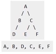
|
ANS 17.
          Minimum Spanning Tree:
A minimum spanning tree of an undirected graph G is a tree formed from graph edges that connects all the vertices of G at lowest total cost. A minimum spanning tree exists if and only if G is connected. Below figure shows the graph which is minimum spanning tree:

-
Using Prim’s Algorithm
-
Kruskal’s Algorithm
ANS 18.
         Dijkstra’s
Algorithm
¨
Solution
to the single-source shortest path problem
in
graph theory
¤
Both
directed and undirected graphs
¤
All
edges must have nonnegative weights
¤
Graph
must be connected
Pseudocode
dist
[s]
←
0
(distance
to source vertex is zero)
for
all
v
∈
V–{s}
do
dist
[v]
←
∞
(set
all other distances to infinity)
S
←
∅
(S,
the set of visited vertices is initially empty)
Q
←
V
(Q,
the queue initially contains all vertices)
while
Q
≠
∅
(while
the queue is not empty)
do
u
←
mindistance
(
Q,dist
)
(select
the element of Q with the min. distance)
S
←
S
∪
{u}
(add
u to list of visited vertices)
for
all
v
∈
neighbors[u]
do
if
dist
[v]
>
dist
[u]
+ w(u, v)
(if
new shortest path found)
then
d[v]
←
d[u]
+ w(u, v)
(set
new value of shortest path)
(if
desired, add
traceback
code)
return
dist
Output
of
Dijkstra’s
Algorithm
¨
Original
algorithm outputs value of shortest path
not
the path itself
¨
With
slight modification we can obtain the path
Value:
δ
(1,6)
= 6
Path:
{1,2,5,6}


No comments:
Post a Comment